Jupyter Notebook - Linear Regression The case solution
Bivariate Analysis
Bi means two and variate means variable, so here there are two variables. The analysis is related to cause and the relationship between the two variables. There are three types of bi-variate analysis.
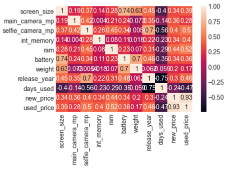
heatmaps
Checking correlations is an important part of the exploratory data analysis process. This analysis is one of the methods used to decide which features affect the target variable the most, and in turn, get used in predicting this target variable.
visualization is generally easier to understand than reading tabular data, heatmaps are typically used to visualize correlation matrices.
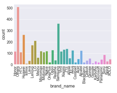
Barplot:
Comparison of brands that users used.
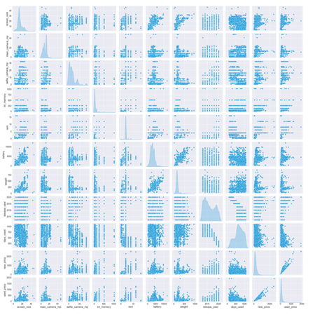
Pairplot:
Relationship between all numeric columns.
Cleaning the Data
Checking for duplicates
We will check if there is any duplicate value exist. If any duplicate value exits we will remove it.
There is no duplicate value exist.
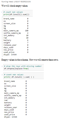
Check Empty Data:
Create a model and fit it
Create a linear regression model and fit it using the existing data.
Let’s create an instance of the class Linear-regression, which will represent the regression model:
Our next step is to divide the data into “attributes” and “labels”.
Attributes are the independent variables while labels are dependent variables whose values are to be predicted. In our datasets, we only have two columns. We want to predict the Used_price depending upon the All colmuns recorded. Therefore our attribute set will consist of the “All colmuns” column which is stored in the X variable, and the label will be the “Used_price” column which is stored in y variable.
Next, we split 0% of the data to the training set while 30% of the data to test set using below code.
The test_size variable is where we actually specify the proportion of the test set.
After splitting the data into training and testing sets, finally, the time is to train our algorithm. For that, we need to import Linear-regression class, instantiate it, and call the fit() method along with our training data.
The linear regression model basically finds the best value for the intercept and slope, which results in a line that best fits the data. To see the value of the intercept and slop calculated by the linear regression algorithm for our dataset.
Now compare the actual output values for X_test with the predicted values, execute the following script:
Luckily, we don’t have to perform these calculations manually. The Scikit-Learn library comes with pre-built functions that can be used to find out these values for us.
Let’s find the values for these metrics using our test data.
The explained variance score explains the dispersion of errors of a given dataset, and the formula is written as follows: Here, and Var(y) is the variance of prediction errors and actual values respectively. Scores close to 1.0 are highly desired, indicating better squares of standard deviations of errors.
Though our model is not very precise, the predicted percentages are close to the actual ones.
Conclusion:
In conclusion, with Simple Linear Regression, we have to do 5 steps as per below:
- Importing the dataset.
- Splitting dataset into training set and testing set (2 dimensions of X and y per each set). Normally, the testing set should be 5% to 30% of dataset.
- Visualize the training set and testing set to double check (you can bypass this step if you want).
- Initializing the regression model and fitting it using training set (both X and y).
- Let’s predict.............................
- Jupyter Notebook – Linear Regression The case solution
- This is just a sample partial case solution. Please place the order on the website to order your own originally done case solution.
Related Case Solutions & Analyses:
 Airbus A3XX: Developing the Worlds Largest Commercial Jet (A)
 Meeting the Diversity Challenge at PepsiCo: The Steve Reinemund Era
 Social media: The New Hybrid Element of the Promotion Mix
 Cirque du Soleil–The High-Wire Act of Building Sustainable Partnerships
 HubSpot: Inbound Marketing and Web 2.0
 Symbian Google & Apple in the Mobile Space (A)
 Sanctuary Soft: International Expansion Strategies
 U.S. Subprime Mortgage Crisis: Policy Reactions (B)
 The Walt Disney Company and Pixar Inc.: To Acquire or Not to Acquire
 HP: The Computer is Personal Again