SPSS Task Case Solution And Analysis, HBR Case Study Solution & Analysis of Harvard Case Studies

Figure 1.2: Scatter plot

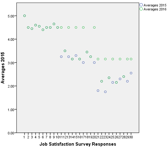
Linear Regression:

Research Question:

Does average job satisfaction level of the year 2015 is a predictor of average job satisfaction level of the year 2016?

Null Hypothesis: Average job satisfaction level of the year 2015 is not a predictor of average job satisfaction level of the year 2016.

Alternate Hypothesis: Average job satisfaction level of the year 2015 is a predictor of average job satisfaction level of the year 2016.

Regression Equation:

Averages 2016 = 1.449 + 0.693 (Averages 2015)

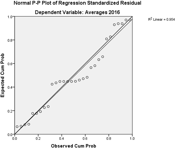
On the basis of p value < 0.001 at 95% confidence level, there has been found the strong statistically significant evidences to reject null hypothesis that states average job satisfaction level of the year 2015 is not a predictor of average job satisfaction level of the year 2016. By accepting the alternative hypothesis that the average job satisfaction level of the year 2015 is a predictor of average job satisfaction level of the year 2016, it has been found that R square is 0.653 that indicates 65.3% data variability around its mean. Coefficient of independent variable 0.693 predict that when a year increases, job satisfaction level increases by 0.693 points while R square shows the accuracy of this prediction which is 65.3%.

Table 1.4: Linear Regression

Model Summary
Model	R	R Square	Adjusted R Square	Std. Error of the Estimate
1	.808^a	.653	.640	.51926
a. Predictors: (Constant), Averages 2015
b. Dependent Variable: Averages 2016

ANOVA
Model		Sum of Squares	df	Mean Square	F	Sig.
1	Regression	14.187	1	14.187	52.618	.000 ^b
	Residual	7.550	28	.270
	Total	21.737	29
a. Dependent Variable: Averages 2016
b. Predictors: (Constant), Averages 2015

Coefficients
Model		Unstandardized Coefficients		Standardized Coefficients	t	Sig.	95.0% Confidence Interval for B
Model		B	Std. Error	Beta	t	Sig.	Lower Bound	Upper Bound
1	(Constant)	1.449	.332		4.368	.000	.769	2.128
1	Averages 2015	.693	.096	.808	7.254	.000	.497	.889
a. Dependent Variable: Averages 2016

Figure 1.3: Normal P-P Plot

One Way Anova:

Research Question:

Is there a significant mean value differences among all three groups in the years 2015 and 2016?

Null Hypothesis: A mean value is same among all three groups in the years 2015 and 2016.

Alternate Hypothesis:A mean value is not same among all three groups in the year 2015 and 2016.

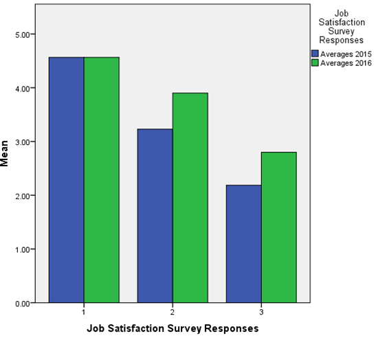
On the basis of p value < 0.001 at 95% confidence level, there has been found the strong statistically significant evidences to reject null hypothesis that states a mean value is same among all three groups in the years 2015 and 2016. By accepting the alternative hypothesis that a mean value is not same among all three groups in the year 2015 and 2016, it has been found that a mean value for three groups in the year 2015 are 4.565, 3.23 and 2.185 respectively while a mean value for three groups in the year 2016 are 4.565, 3.9 and 2.8 respectively.

Table 1.5: One Way Anova

Descriptive
		N	Mean	Std. Deviation	Std. Error	95% Confidence Interval for Mean		Minimum	Maximum
		N	Mean	Std. Deviation	Std. Error	Lower Bound	Upper Bound	Minimum	Maximum
Averages 2015	1	10	4.5650	.16841	.05326	4.4445	4.6855	4.40	5.00
	2	10	3.2300	.16533	.05228	3.1117	3.3483	3.00	3.50
	3	10	2.1850	.24950	.07890	2.0065	2.3635	1.75	2.55
	Total	30	3.3267	1.00899	.18422	2.9499	3.7034	1.75	5.00
Averages 2016	1	10	4.5650	.16841	.05326	4.4445	4.6855	4.40	5.00
	2	10	3.9000	.64205	.20303	3.4407	4.3593	3.15	4.50
	3	10	2.8000	.45704	.14453	2.4731	3.1269	2.15	3.15
	Total	30	3.7550	.86576	.15807	3.4317	4.0783	2.15	5.00

ANOVA
		Sum of Squares	df	Mean Square	F	Sig.
Averages 2015	Between Groups	28.462	2	14.231	361.978	.000
	Within Groups	1.061	27	.039
	Total	29.524	29
Averages 2016	Between Groups	15.892	2	7.946	36.702	.000
	Within Groups	5.845	27	.216
	Total	21.737	29

Post Hoc (Tukey) Tests shows the multiple comparisons of all groups for both of the years and indicates that there is a significant mean differences among all groups at 0.05 significance level. By comparison of group means from 2015 to 2016, group 1 shows no difference in the mean from 2015 job satisfaction level to 2016 job satisfaction level while there has been found a difference between two years group means for group 2 and 3 as it can be seen in figure 1.4.

Table 1.6: Post Ho c Tests

Dependent Variable	(I) Job Satisfaction Survey Responses	(J) Job Satisfaction Survey Responses	Mean Difference (I-J)	Std. Error	Sig.	95% Confidence Interval
Dependent Variable	(I) Job Satisfaction Survey Responses	(J) Job Satisfaction Survey Responses	Mean Difference (I-J)	Std. Error	Sig.	Lower Bound	Upper Bound
Averages 2015	1	2	1.33500^*	.08867	.000	1.1151	1.5549
	1	3	2.38000^*	.08867	.000	2.1601	2.5999
	2	1	-1.33500^*	.08867	.000	-1.5549	-1.1151
	2	3	1.04500^*	.08867	.000	.8251	1.2649
	3	1	-2.38000^*	.08867	.000	-2.5999	-2.1601
	3	2	-1.04500^*	.08867	.000	-1.2649	-.8251
Averages 2016	1	2	.66500^*	.20808	.010	.1491	1.1809
	1	3	1.76500^*	.20808	.000	1.2491	2.2809
	2	1	-.66500^*	.20808	.010	-1.1809	-.1491
	2	3	1.10000^*	.20808	.000	.5841	1.6159
	3	1	-1.76500^*	.20808	.000	-2.2809	-1.2491
	3	2	-1.10000^*	.20808	.000	-1.6159	-.5841
*. The mean difference is significant at the 0.05 level.

Figure 1.4: Bar Chart

This is just a sample partical work. Please place the order on the website to get your own originally done case solution.