Matlab Analysis Of Drying Colloidal Film Case Solution And Analysis, HBR Case Study Solution & Analysis of Harvard Case Studies

Matlab Analysis Of Drying Colloidal Film Case Solution

Introduction

The drying of colloidal film is given importance in many areas especially in painting and coating. The spatial distribution of colloidal particles in the drying process is determined by tow competing process. One is Brownian motion while the other is evaporation. In this work we performed the analysis of wide spread evaporation of colloidal film at both the initial and boundary conditions. Following the aspect, we developed a code o MATLAB to solve the partial differential equation of the colloidal transport equation.

Literature Review

Brownian motion

Hydrodynamic Collisions are described in terms of Brownian motion when two fluids collide, and have different viscosities and pressures. Brownian flow in a dilute droplet of water. The effect of Brownian motion in an unstable fluid with constant macro particles in a suspended fluid with fixed macro objects.
Brownian motion in an unconfined fluid, where it is assumed that a fluid flows with viscous friction at constant velocity and constant volume. The boundary layer of a fluid is known as Brown's Law and it describes the velocity distribution, the velocity gradient and velocity stability of a system. Brown's Law predicts that the pressure and volume of a fluid will be proportional to the density of the fluid. It also predicts that a fluid of constant viscosity, that is, of the same temperature, will not expand or contract.

Colloidal Film

Colloidal suspensions are frequently used as thin films on substrates to modify or enhance their surface properties. A familiar example is latex paint, which, by changing the corrosion resistance and color of the surface, makes the material more durable and aesthetically appealing.

When thin films of colloidal fluids are dried, a range of transitions are observed and the final film profile is found to depend on the processes that occur during the drying step. This article describes the drying process, initially concentrating on the various transitions. Particles are seen to initially consolidate at the edge of a drying droplet, the so-called coffee-ring effect.

Dispersion

In Hydrodynamic systems, the pathogen and dissolved material interact via hydrodynamic forces. The forces depend on the size, shape and composition of the contaminated reservoir. A model is usually set up that assumes that the pathogen is a solid particle and is traveling at the same velocity and in the same direction as the particles in the reservoir. These models do not include any hydrodynamic effects of suspended solids. They only consider the particles in the reservoir.

Discursive models that include an eddy flow are more accurate than dispersion models that do not include an eddy flow and do not include an effect of the pathogen on the reservoir surfaces. In a dispersion model, the pathogen is considered to act as a viscous fluid, and not a solid particle.

The dispersion model is used to determine the effects of gravity and hydro-static forces on the position and velocity of a fluid mass in a reservoir. The model is applied to calculate the time delay in the reaction of a fluid to a force applied to it.

Task 1

Matlab Code

n= 1E4;

x = linspace(0,n,10);

t = linspace(0,0.5,50);

m = 1;

pe=10;

sol = pdepe(m,@pdefun,@pdeini,@pdeboun,x,t);

u = sol(:,:,1);

plot(x,u)

xlabel('x')

ylabel('Solution u(x,t)')

title('Solution of PDE')

function [c,f,s] = pdefun(x,t,u,dudx)

c = 1;

f = ((1/0.1)*(1-t)^2).*dudx;

s = -(x/(1-t)).*dudx;

end

function u0 = pdeini(m,n,Pe,u0)

u0=0.01;

end

function [pl,ql,pr,qr] = pdeboun(xl,ul,xr,ur,t)

pl = ul;

ql = 0;

pr = 0.1*(1-t)*ur;

qr = 0;

end

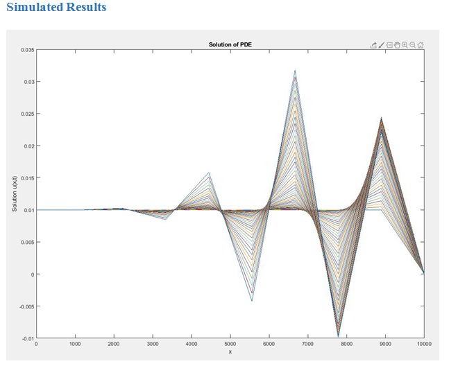
Task 2