Cleaning & Processing of Raw Data Set
In deliverable 1 of this project, we have identified a number of the issues with the data set. The first issues related to the presence of the unusual values or called as outliers in the data set. The interquartile range had been calculated and based on the lower fence and the upper fence intervals we have identified a number of variables where the outliers were present including the dependent variable which is the rate of crime in small US cities represented by Y. All those variables which had outliers in their data are Y, X1, X2, X5 and X6. If we compare the lower and the upper fence with the raw data as present in the data set file, then we can identify all the outliers which are out of the lower and the upper fence for each variable.
Therefore, first thing we did is to clean the entire data set and remove all the outliers to create a new trimmed data set. The trimming of the data set and the removal of all the lower and higher value outliers has been done through Winsorization. Winsorization is the transformation of the statistical data sets by limiting the extreme values within the data set in order to reduce the effect of the spurious outliers for performing the exploratory analysis in deliverable 3 of the project. In Winsorization all the high extreme values have been replaced by the upper bound value of that particular variable and the lower extreme values have been replaced by the lower bound value. The trimmed data set could be seen in the excel spreadsheet. The comparison of the means and the standard deviation for all the variables between raw data set and trimmed data set is shown in exhibit 1 in the appendix. Specifically the standard deviations show the effect of the removal of outliers from the data set. The trimmed data set could now be checked for extreme values by looking at lower and upper bounds as shown in exhibit 2 in the appendix.
Another important assumption for performing the exploratory analysis such as regression analysis is that the dependent variable should be normally distributed. This assumption has been tested and the normal curve in exhibit 2 in appendix shows that the dependent variable is normally distributed. Therefore, this shows that the Y variable could be used as an independent variable in our further exploratory analysis such as multiple regression analysis. It should be noted that the mean of the normal curve has decreased and the standard deviation for the normal curve has also decreased. This shows that the dependent variable data is now more accurately distributed as seen by the normal curve in exhibit 3 in the appendix.
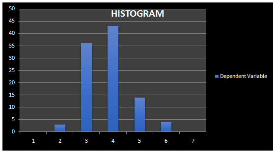
Finally, we have also identified certain data entry issues with respect to the dependent variable which is crime rate. The previous histogram based on the raw data set showed a rightly skewed histogram which meant that the mean was greater than the median of the dependent variable. The right skewed distribution of the dependent variable would have distorted the results of regression analysis. This might have also been due to the presence of the outliers in the data set. The new histogram for the dependent variable Y based on the trimmed data set shows that the histogram is normally distributed now as the curve shows exactly a bell shaped curve. This shows that the effects of extreme values have been cleaned in the data set and points occurring on one side of the mean are similar as on the other side. The histogram could be seen in exhibit 4 in appendix. The data has been processed; the descriptive statistics and the final data set for performing the exploratory analysis could be seen in the data file.
Appendix
Exhibit 1: Trimmed Data Set Means
| RAW DATA VS TRIMMED DATA SET | |||||||
| Y | X1 | X2 | X3 | X4 | X5 | X6 | |
| Mean (Raw Data) | 682.65 | 568.21 | 36.85 | 58.16 | 15.33 | 28.64 | 13.98 |
| Mean (Trimmed Data) | 667.57 | 542.77 | 35.95 | 58.16 | 15.33 | 27.80 | 13.77 |
| Stdev (Raw Data) | 219.38 | 425.27 | 10.13 | 8.19 | 4.59 | 10.92 | 3.88 |
| Stdev (Trimmed Data) | 166.99 | 301.68 | 6.99 | 8.19 | 4.59 | 7.93 | 3.06 |
Exhibit 2: Checking Outliers
| OUTLIERS IN DATA (Check with Trimmed Data) | |||||||
| Y | X1 | X2 | X3 | X4 | X5 | X6 | |
| Quartile 1 | 546.75 | 325.75 | 31 | 51.75 | 12 | 23 | 12 |
| Quartile 3 | 776 | 723.25 | 40 | 65 | 18 | 32 | 16 |
| Interquartile Range | 229.25 | 397.5 | 9 | 13.25 | 6 | 9 | 4 |
| Upper Bound | 1119.875 | 1319.5 | 53.5 | 84.875 | 27 | 45.5 | 22 |
| Lower Bound | 202.875 | -270.5 | 17.5 | 31.875 | 3 | 9.5 | 6 |
| Outliers | Does Not Exist | Does not Exist | Does not Exist | Does not Exist | Does not Exist | Does not Exist | Does not Exist |
Exhibit 3: Normal Distribution Curve
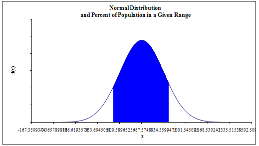
Exhibit 4: Dependent Variable Histogram
Related Case Solutions & Analyses:
 Solutions For Customer Complaints About Offshoring And Outsourcing Services
 Investment Technology Group
 Operational Capabilities: Hidden in Plain View
 Retail Relay A
 Threat of Terrorism: Epilogue
 Publishing Group of America (A)
 Explore Inc.
 MarketSoft
 Georges T-Shirts Addendum
 Eco7: Launching a New Motor Oil